Moving on up:
A couple of summers ago I experimented with a satellite dish antenna
that was not receiving a signal where there should have been one. At
the time I
did not know how to test the antenna to determine whether it measured
up to published
specifications. It seemed possible that something could have shorted or
failed in an
inaccessible part of the structure. My antenna analyzer was of no use.
The maximum
frequency that it could
generate or scan is 230 MHz, far below the
microwave range. Thus, I became curious about vector network analyzers,
specifically those
that operate at gigahertz frequencies. A cursory
Internet search sufficed to dismiss that idea. Such
instruments cost thousands of dollars. —I moved on to other projects.
Not much had changed in regard to bench
instruments and their
cost the next time I
became curious about
VNA’s. There was one
outlier, however, a pocket-size ‘instrument’ that
sold for less than $100 and claimed to work from 50 KHz to 900 MHz, and
even in one model to 1.5 GHz. My thought was not that 1.5 GHz is far
below 6 GHz, but rather that 1.5
GHz is a great deal
higher than 230 MHz, and
for an unbelievably low cost, compared to professional VNA’s.
That particular glass was half full.
Nearly everything in the box (photo)
came with the unit, except the 3D printed touchscreen stylus (this
one), and the large coax adapters stowed underneath the clear
plastic tray. Accessories include three SMA male calibration
connectors, one SMA female barrel connector, two short SMA jumpers, and
a USB-C interface/charging cable. The kit also includes a
single-sided fold-out menu diagram, without which it is easy to get
lost, until the menu structure becomes familiar.
Small steps: Having no previous experience with a VNA,
I had trouble at first making sense of the display, even for
calibration. There is no book. And the usefulness of relevant Internet
resources varies. I found this manual by Gunthard Kraus DG8GB to
be most helpful, although parts of it are beyond my present
understanding.
 As if learning to perform and interpret NanoVNA measurements were
not challenging enough, the instrument seemed to have a mind of its
own, spontaneously jumping over submenus, sometimes reaching an obscure
end branch of the menu tree. While the stylus worked much better than
my finger, the touch screen had to be touched just
right, not tapped or long-pressed. The multifunction switch
also
exhibited the jitters. I wanted to call it the ‘malfunction’ switch. It
responded like a worn joystick. If precisely the right
amount of pressure were applied in a magic direction the
multifunction switch would sometimes do what was expected. More often
the screen would jump to some unwanted option. —That is when the
USB cable became a crucial accessory.
As if learning to perform and interpret NanoVNA measurements were
not challenging enough, the instrument seemed to have a mind of its
own, spontaneously jumping over submenus, sometimes reaching an obscure
end branch of the menu tree. While the stylus worked much better than
my finger, the touch screen had to be touched just
right, not tapped or long-pressed. The multifunction switch
also
exhibited the jitters. I wanted to call it the ‘malfunction’ switch. It
responded like a worn joystick. If precisely the right
amount of pressure were applied in a magic direction the
multifunction switch would sometimes do what was expected. More often
the screen would jump to some unwanted option. —That is when the
USB cable became a crucial accessory.
Exercise 1 - VSWR: It is usually a good idea when
exploring
something new to start with a simple example. I chose VSWR for a first
real-world measurement, after testing with the calibration connectors.
By
chance an antenna that I’d used in an unrelated project
sat on the computer desk.
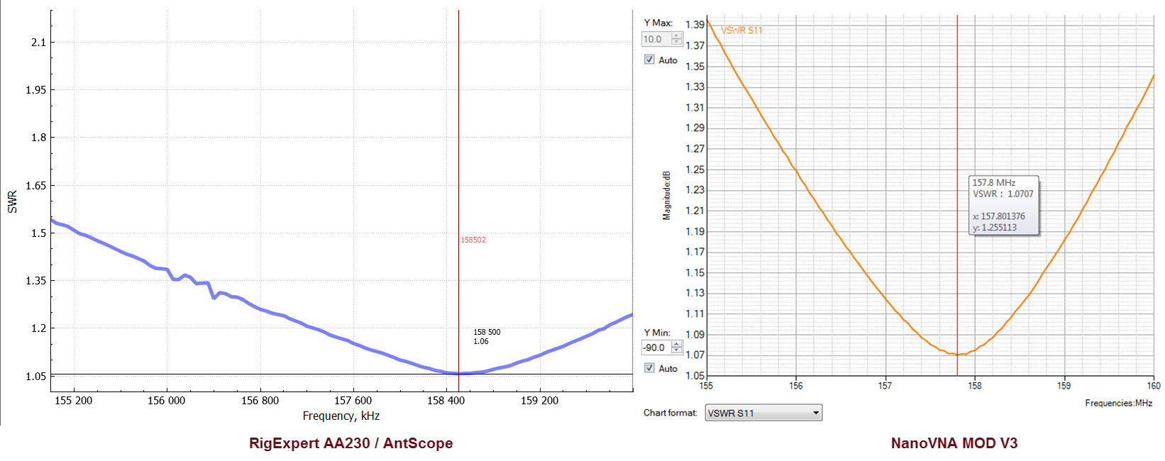
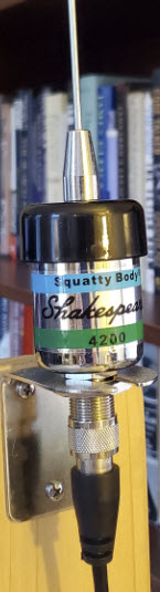
It was a Shakespeare marine antenna, designed to be mounted on the
masthead of a sailboat. I connected the antenna to CH0 of the NanoVNA
using a 3-foot length of RG58 and a 6-inch SO-239 to SMA female
adapter. The sweep range was centered on the marine VHF band. Later I
used the
RigExpert
AA230 antenna analyzer to measure
the same antenna, in the same physical place, and
with the same RG58 jumper (but without the SMA adapter). These
measurements are shown side-by-side below.
The y-axes
are scaled differently, because I did not realize when scaling the
NanoVNA MOD v3 graph that the
(RigExpert) AntScope2 graph could not be
scaled in the same
way. I cannot explain why the NanoVNA software label for
the y-axis says dB—SWR is a ratio, not a logarithm. Also,
the exact frequency of
minimum VSWR is
different between the two measurements. That could be due
to the slightly different hookup (SO-239 to SMA part), or it could be a
calibration issue. In any case the curve is quite flat (VSWR <
1.2 : 1) in that part of the range, so the difference is not
significant.

Prior to testing
the Shakespeare antenna
for this exercise I had supposed that marine masthead antennas are not
much good, basically that they rely on height and possibly also on the
mast itself (counterpoise) for their performance. However, VSWR
measurements from both instruments indicate that this antenna is well
matched at the marine VHF band. The moral is that a perfectly good
marine VHF antenna should not be wasted on a non-floating piece of
furniture.1
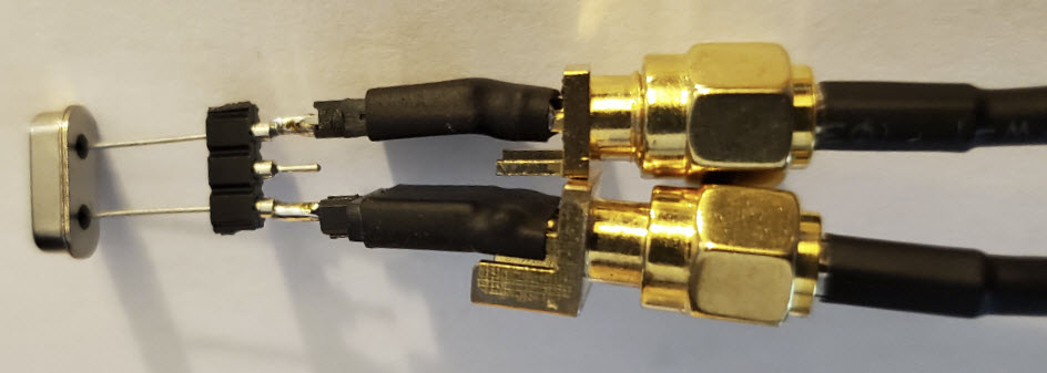 Exercise 2 - Parameters of a crystal: While an antenna
analyzer has a single RF port, a vector network analyzer has two or
more. In the NanoVNA, CH0 is
the signal source and is also used in measuring reflections. CH1 is the
input or receive port when the signal source is transmitted through an
external circuit. The two jumpers supplied with the NanoVNA are used to
connect the device under test with the NanoVNA source and receive
ports. I thought a crystal would be the simplest thing to measure using
the two ports. It could be plugged directly into the ports using a
simple jig (photo)—the female SMA sockets on the device itself are a
little more than 3 cm apart, too far to plug the crystal
directly into the device.
Exercise 2 - Parameters of a crystal: While an antenna
analyzer has a single RF port, a vector network analyzer has two or
more. In the NanoVNA, CH0 is
the signal source and is also used in measuring reflections. CH1 is the
input or receive port when the signal source is transmitted through an
external circuit. The two jumpers supplied with the NanoVNA are used to
connect the device under test with the NanoVNA source and receive
ports. I thought a crystal would be the simplest thing to measure using
the two ports. It could be plugged directly into the ports using a
simple jig (photo)—the female SMA sockets on the device itself are a
little more than 3 cm apart, too far to plug the crystal
directly into the device.
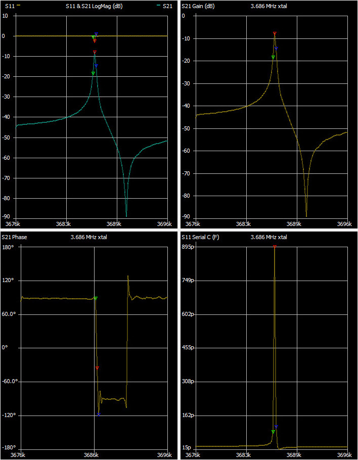
It is possible to read measurements
directly from the small VNA screen, but this is not easy—the NanoVNA is
not a bench instrument. However, the computer applications that
complement the NanoVNA not only graph data in user-selectable formats,
but also perform analyses and calculate characteristic parameter
values. The graphs
above depicting selected measurement results for a 3.686 MHz crystal
were produced by an application called NanoVNA-Saver.
The three colored markers were placed automatically by the program.
Each of these markers is associated with a block of measurement data.
(not shown).
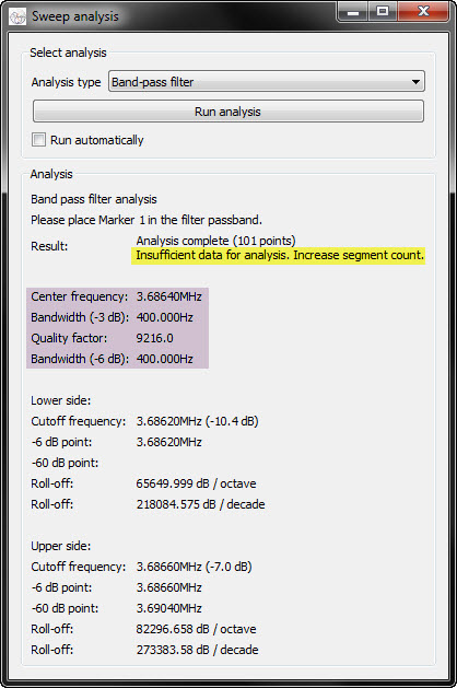
I also exercised the ‘Analysis’
function of the NanoVNA-Saver application using this same crystal, and
later with another higher frequency crystal (22.1184 MHz). The
‘Insufficient data’ warning (yellow) was puzzling at first. Wouldn’t
100 points
be sufficient for a 20 KHz sweep? That number equates to 200
Hz between each pair of points, which makes the 3 dB bandwidth
just 2 points wide, so perhaps not.
Clearly, the observed center frequency
necessarily depends on the NanoVNA’s frequency calibration. Finally,
given that crystals have a narrow bandwidth and high Q, these
measurement results are
not necessarily surprising or significant, but may serve to
demonstrate some of the instrument and computer software
capabilities.
Exercise 3 - Filter: There are no
manufactured band-pass filters or IF transformers etc. in
my old parts bin. So I thought maybe I could learn something by making
one. This QST
article from 1988 describes a 3-pole Butterworth filter, and includes
a table of component values for each of the traditional HF ham bands
160 - 10
meters. The original article
was aimed toward construction of high-power transmitter
filters. And surely to make a useable RF band-pass filter it would be
necessary to
respect component values, construction techniques, shielding, etc.
However, my
goal was not to make a functional transmitter filter, but rather to use
the canonic design and related component values as a bridge to another
nanoVNA measurement exercise. I
thought it should be possible to visualize the pass band graphically,
and to exhibit properties of the filter that depend on L and C values,
but substituting low-voltage components.
I first assembled the circuit on a
breadboard. However, the inevitable loose connections made it difficult
to
obtain reliable measurements, so I transferred everything to a
perforated board (photo), substituting a small trimmer capacitor for C2
in the circuit diagram. Capacitance and inductance values were taken
from the 7
MHz row of Table 1 in the QST
article. However, as previously
noted I did not have the same toroids as recommended in the article.
Instead I used a small iron powder form that was on hand
(T37-6), and a free
application called mini Ring Core Calculator to
compute the number of turns needed to produce tabled inductance values.
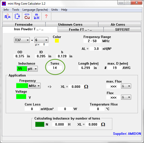

The
illustration above shows an example calculation that computes the
number of turns for L1 and L3, each 0.55 μH (Table 1 in the QST article). I
should mention that I also experimented with ferrite toroids, but could
not hit desired inductances dead-on with these. Overshooting the number
of turns is not a big deal when
winding inductors,
because turns are easily removed. The opposite is not true, however.
That is part of the reason why a 120 pF trimmer was substituted for C2
(100 pF in the table). I did not use high tolerance capacitors, and
found that adjusting this capacitance would
slide the pass band one way or the other, to yield a more nearly
centered
measurement result.2
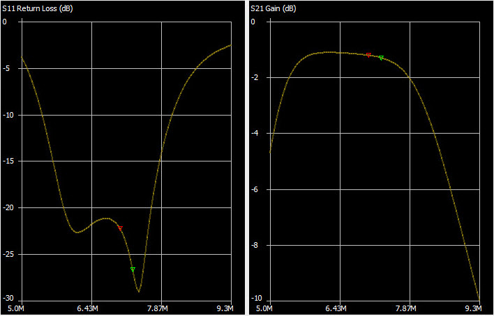
Once again the results surprised me.
Only one
measurement indicated a narrow pass band that approximately coincided
with the 7 MHz ham band. That specific
measurement could not be reproduced, so I am omitting it. Most
replications produced results resembling the diagrams above, where the
pass band is roughly 2 MHz wide. And what is that wobble in the ‘Return
Loss’
diagram? —Perhaps it has something to do with reflection
(left graph) versus through-filter
(right graph) measurements.
Because of such dangling questions the
exercise was not wholly satisfying.
True, the test filter substantially attenuates frequencies above and
below the pass band, which would suffice to provide a degree of
isolation between bands. On the other hand I had pictured a narrower
pass band, with cutoffs nearer the 40 meter band edges [colored
markers]. Maybe that is
where additional filter stages would be indicated. Clearly
there is much to learn!
Demo
video: [forthcoming, or maybe not]
1. Of course, a satisfactory impedance match does not in itself imply that the antenna radiates efficiently.
2. Ferret image from Wikimedia Commons.
Project descriptions
on this page are intended for entertainment only.
The author makes no claim as to the accuracy or completeness of the
information presented. In no event will the author be liable for any
damages, lost effort, inability to carry out a similar project, or
to reproduce a claimed result, or anything else relating to a decision
to
use the information on this page.