Oscilloscope Math Mode, tinySA Ultra RF power measurement, tinySA
signal generation, filter testing
These studies were prompted by a
remark from a respected source, claiming that an oscilloscope’s FFT1 function could
not be trusted for
measuring low pass filter parameters (in the HF regime). An
oscilloscope is not a spectrum analyzer. Would
selected
measurements with a consumer grade oscilloscope’s math
mode reveal inconsistencies, or otherwise call into question the
instrument’s accuracy or reliability?
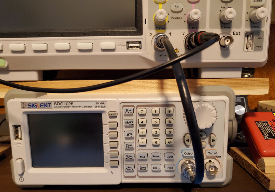
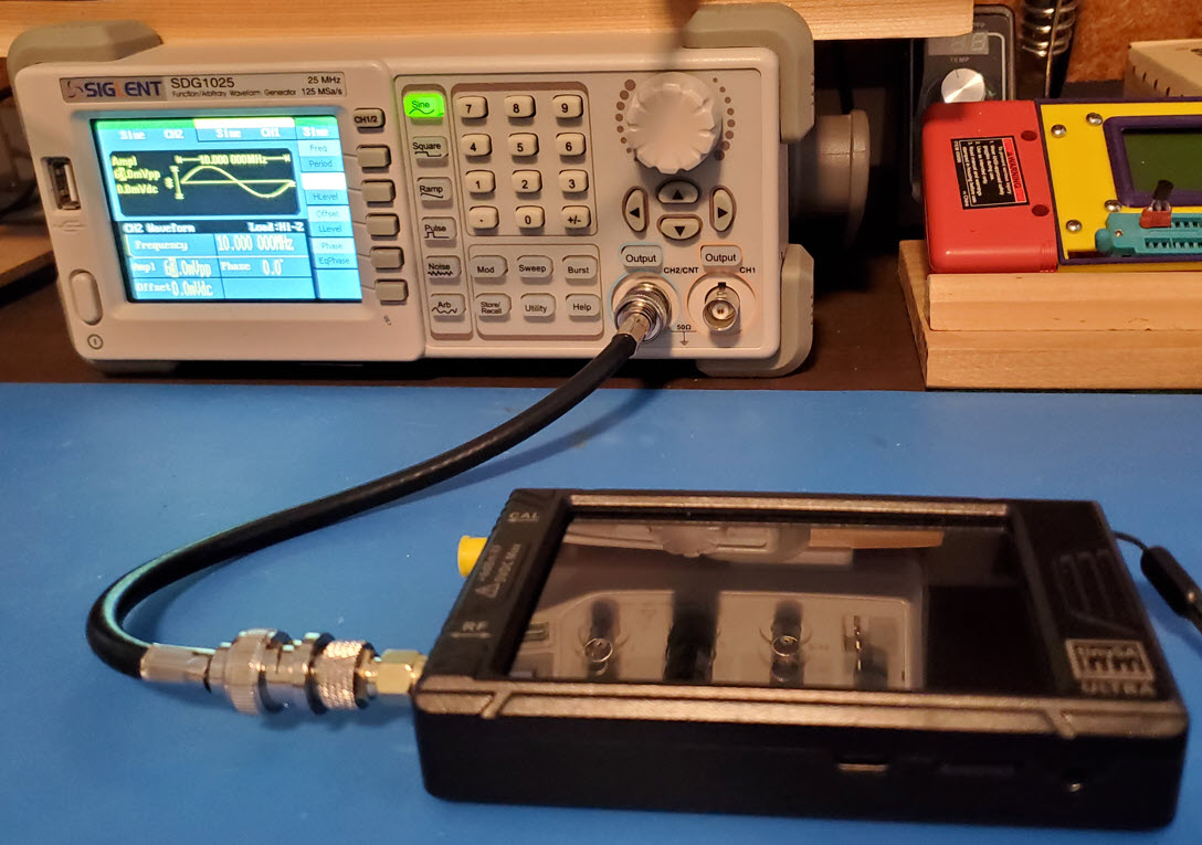
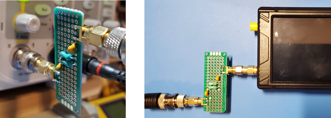
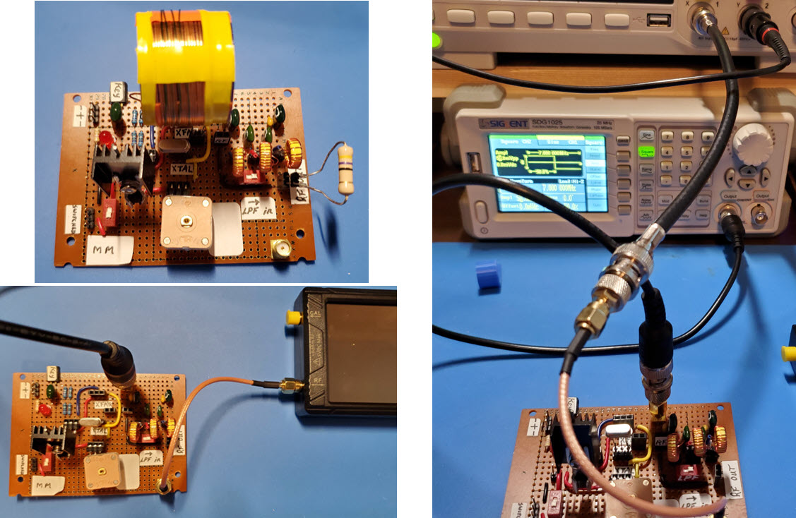
Exercise 1: The setup for this exercise is pictured above.
The Siglent signal generator’s output was jumpered directly to the
oscilloscope’s input using a short piece of 50 ohm coax terminated on
both ends with male BNCs. Three power levels: -10 dBm, -20 dBm, and -30
dBm were crossed with four frequencies: 5, 10, 15, and 20 MHz for
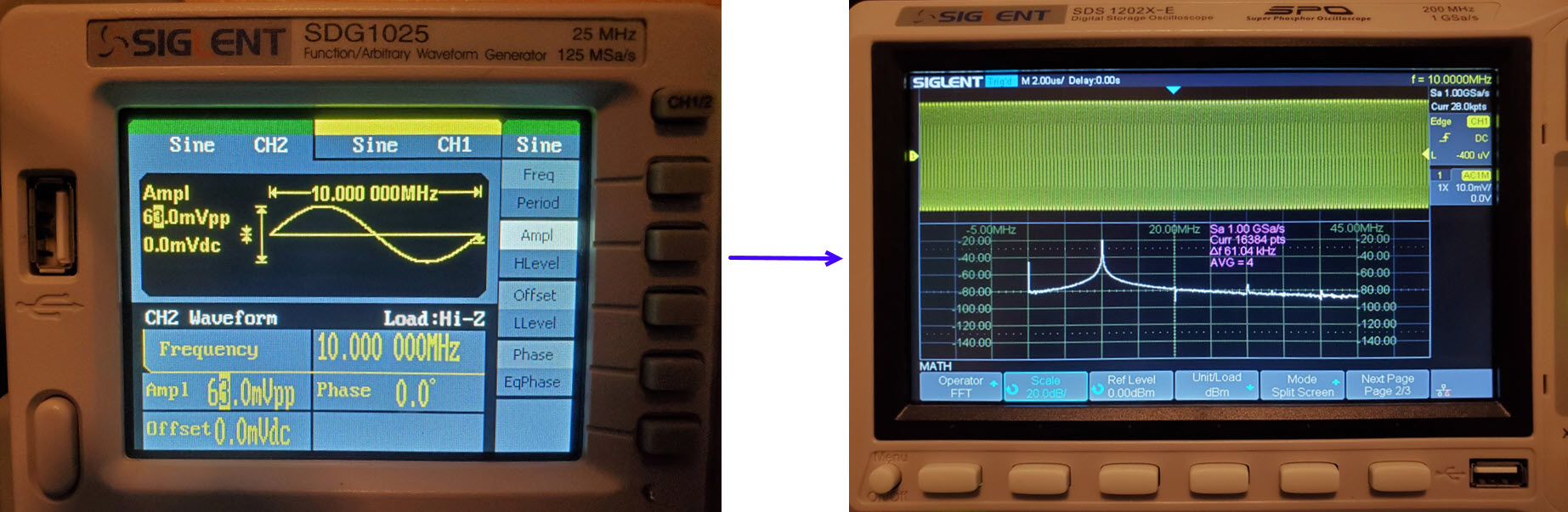
testing. In the illustration below, the signal generator is set to
produce a 10 MHz sine wave at 63 mV peak-to-peak. This output voltage
corresponds to
the -20
dBm power level at 50 ohms.2
It would be pointless to
reproduce a table of results, as the measurement for each power level
was the same as the stimulus power (output of function generator). Oscilloscope measured power at a given
source level did not vary across the 5 to 20 MHz test frequency range.3
Exercise 2:
Along with the advice not to rely on oscilloscope FFT
mode was an
alternative suggestion to use a spectrum analyzer, minimally an
inexpensive tinySA, for making filter measurements. This second exercise examines the tinySA
Ultra for the same
power × frequency values used in Exercise 1. The physical setup is
almost identical, except that a slightly longer length of coax was used,
and the spectrum analyzer end included a BNC-to-SMA adapter.
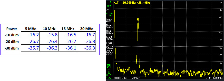
The same 12 measurements were carried
out using the
tinySA Ultra. It would be possible to dispense with a table of
measurements for this study as well. However, the illustration below
shows the values obtained for each combination of power and frequency,
as well as a screen capture of the representative 10 MHz at -20 dBm
signal as received by the tinySA Ultra. Measures averaged -6.35 dBm
from the stimulus power value. In other words, tinySA Ultra reported
the
signals to be consistently weaker than their programmed (and
oscilloscope-measured)
values by about 6⅓ dBm. Otherwise
measurements were consistent between power levels and across
frequencies.
Exercise 3:
The tinySA is two instruments in one. In addition to its spectrum
analyzer function the unit can also be used as a signal generator.
However, in that application it is limited a producing a sine wave
signal at a specified power level—It does not generate other waveforms,
as a function generator would. Nor is the output level as finely
adjustable as the bench instrument’s is.
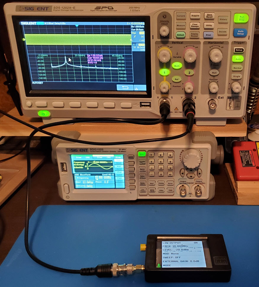
The photo above shows the setup for this
exercise. Although the bench function generator is powered-on, its
outputs are not connected and it is not involved in the exercise.
Instead, the tinySA is directly connected to the oscilloscope. Coax and
adapter are the same as in the previous exercise, but this is a
different tinySA, the basic model, not Ultra. It should be possible to
read test values from the photo. Output is a -20 dBm sine wave at 10
MHz. The oscilloscope trace reads above the -20 dBm grid line,
about ¼ up toward the 0 dBm reference level, which would make it about
-15 dBm. This is consistent with the previous exercise. Readings at the
other test frequencies were similarly around 5 to 6 dB stronger than
advertised. For example, here is the 15 MHz measure:
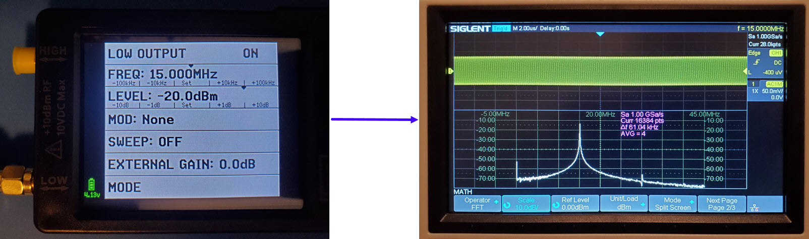
Although the tinySA is not as versatile as the bench
function generator, it has one capability that the Siglent instrument
lacks. tinySA can generate signals in the VHF and even UHF ranges while
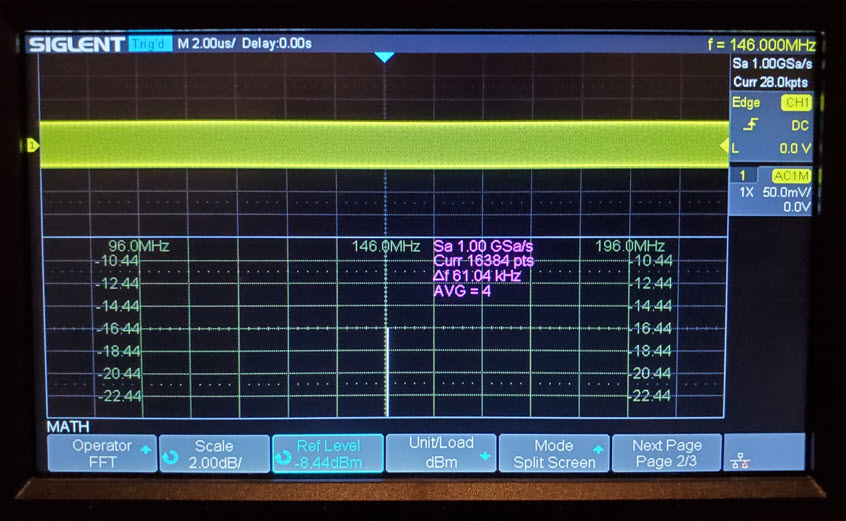
the maximum frequency of the bench instrument is 25 MHz. I was curious
as to how the oscilloscope would fare in measuring the power of a 2
meter band signal. This was not an idle curiosity as I had carried out
some preliminary tests in the VHF domain, and was contemplating another.
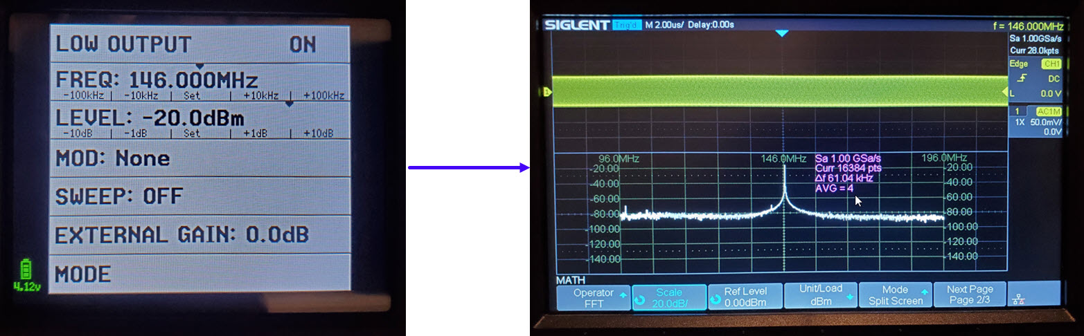
To zero-in on the oscilloscope’s power
measurement at higher precision, I temporarily adjusted the vertical
scale and
allowed the reference level to float. The downside was that the noise
floor could no longer be seen, as noise power fell below the zoomed
display range. On the other hand, the more precise numeric value for
signal power -16.44 dBm was close to the one interpolated for readings
in the HF range (photo below). While it may be optimistic to hope that
tinySA’s generated signal power remains the same at all frequencies,
the fact that the oscilloscope measured a more-or-less constant value
from HF to VHF suggests that generated power is approximately constant
across this much used part of the spectrum. The bane of these
measurements is that we don’t know which instrument has the true or
more nearly true dBm value.
The score is two to one in favor of the function
generator’s output reporting true power, -10 dBm, -20 dBm and -30 dBm,
in that both Siglent bench instruments agree, and neither agrees with the
tinySA.
Exercise 4: Setting aside the puzzling difference in
absolute power measure between the oscilloscope and tinySA, and
recalling that the context of the original motivating issue was filter
measurement, this exercise focuses on the measurement of harmonics and
their relative attenuation with respect to a fundamental. For this and
the next two exercises the source signal, i.e., the fundamental, was a
square wave at 7 MHz. I adjusted the function generator’s output to
produce a -20 dBm measure at the oscilloscope. For this measurement the
power scale was temporarily adjusted as before in order to be read with greater precision (not shown). A square wave of 55 mV
P-P sufficed to produce a -20 dBm reading.
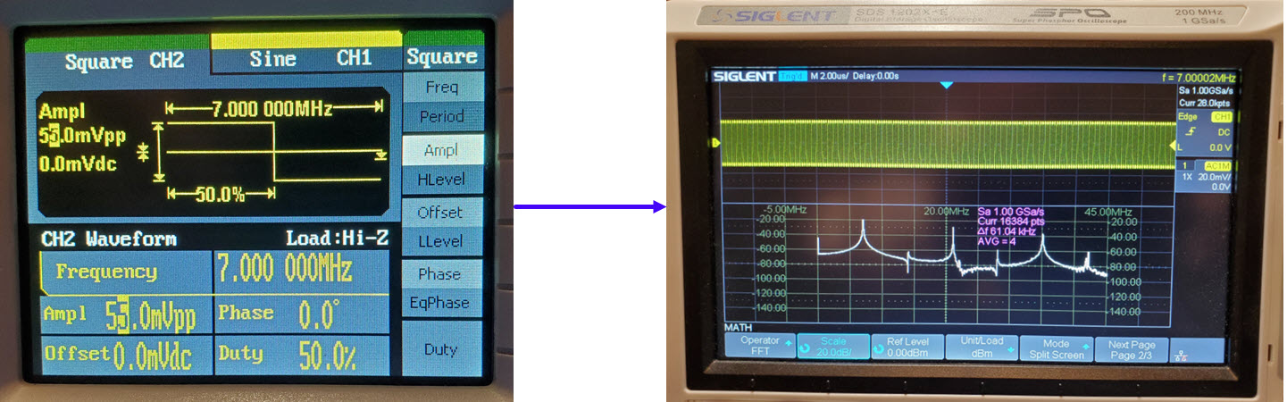
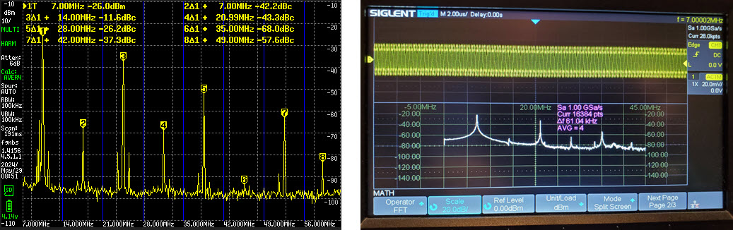
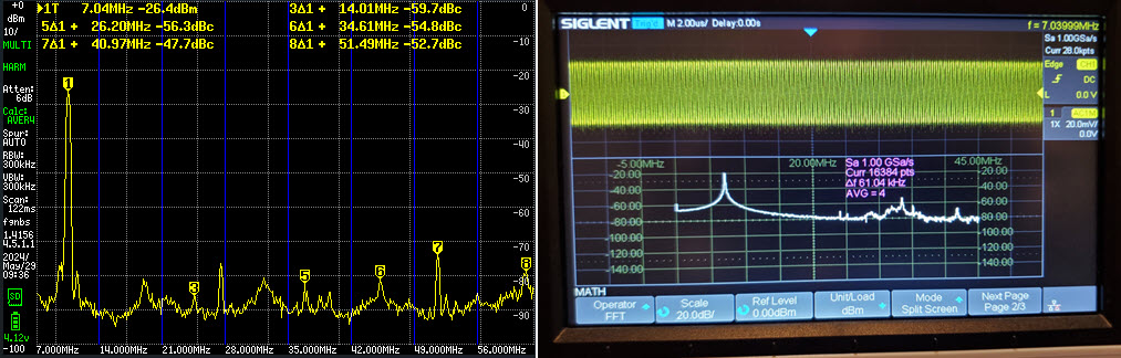
The generated square wave produced
significant harmonics, as expected (above right). The 21 MHz harmonic looks to be at
about the -30 dBm dotted line, while the 35 MHz harmonic is just above
the -40 dBm grid line, roughly -38 dBm. The next part of this exercise
was to observe the same signal on the tinySA Ultra. A neat feature of
the tinySA is its harmonic measurement mode. In this measurement mode,
the unit puts markers on each harmonic peak and displays numeric power
deltas. One other difference is that after the fundamental frequency
and measurement span have been specified,
tinySA adjusts the display range automatically. Evidently the term ‘span’ in
this context refers
to the span above the fundamental, not to the total display width. The
side-by-side image below shows tinySA’s normal spectrum display (left)
and the harmonic measurement display (right).
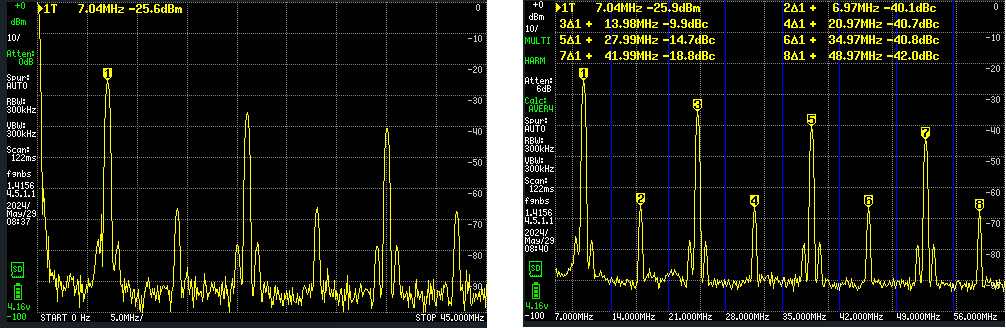
Note that the fundamental was measured to be -25.6
to -25.9 dBm, or roughly 6 dB weaker than the corresponding
oscilloscope measure, same as in the preceding sine wave exercises.
tinySA’s harmonic measurement display confused me at first. Numeric
frequency numbers are offsets from the fundamental frequency, not
absolute frequencies. Thus marker 3∆1 refers to 7 MHz + 14 MHz = 21
MHz; similarly marker 5∆1 refers to 7 MHz + 28 MHz = 35 MHz. The 21 MHz
(true frequency) harmonic is measured at -9.9 dBc and the 35 MHz
harmonic at -14.7 dBc.4 Textual labels at the bottom of the graph are also confusing. These refer
to the harmonic frequencies not to nearby grid lines. All this is
probably well-understood by experienced users of the TinySA (or other
spectrum analyzers) but was new to me.
If absolute power values are ignored and only
harmonic suppression values considered, the 21 MHz harmonic suppression
is essentially identical to the oscilloscope measure, and the 35 MHz
one about 3 dB stronger (less suppressed) as measured by tinySA.
However, it should be noted that the oscilloscope estimates were made
by eye at a coarse scale (20 dB/scale division).
Exercise 5: This exercise and the next one dip into filter
testing. The first test ‘filter’ (not really proven to be a filter at
this point) was a 3-component low pass Chebyshev type, two capacitors
and an
inductor. The filter was connected either to the oscilloscope or tinySA
Ultra using the same coax jumper as in the previous exercise, with a
suitable adapter on the instrument end.
Two questions spring to mind. First does the filter
do anything? That question is most easily assessed by comparing tinySA
harmonic deltas measured with the filter IN to those with the filter
OUT (Exercise 4). The stimulus (source signal) is the same in both
measurement setups, a 7 MHz square wave and -20 dBm or -26 dBm power
level, depending on which instrument you believe. Based on this comparison the
putative low pass filter does seem to do something. Its effect is
most pronounced at 35 MHz and above. The 3∆1 measure (21 MHz true)
decreases by a mere 1.7 dB, while the 5∆1 measure (35 MHz harmonic)
decreases by 11.5 dB, that is from around -40 dBm to -50 dBm.
The second question that can be addressed in this
rather crude filter context is whether the oscilloscope agrees with the
tinySA Ultra, in regard to the relative effect of the filter. Does the
oscilloscope show a similar trend to the one outlined in the previous
paragraph? Although the scale is coarse in the oscilloscope screen
image (right-hand photo above), the 15 MHz harmonic power decrease is
in approximate agreement with the same from tinySA. At 15 MHz the
oscilloscope trace peak falls just below the -30 dBm dotted line (or
roughly 11 dB below the fundamental). The 35 MHz oscilloscope peak
falls just above the -60 dBm grid line, not quite 40 dB below the
fundamental. Without the filter, the oscilloscope had indicated just
above the -40 dBm grid line for this harmonic (first photo in Exercise
4). The change from filter OUT to filter IN is roughly -20 dB. In
summary, the general form of the filter effect is the same for
both instruments, but both absolute power measures and deltas differ to
an extent.
Exercise 6: I recalled having made a 3-stage low pass
filter for 7 MHz, and thought that it had been constructed as a
separate
plugin unit—in fact I was sure it had. However, I have not been able to
locate that construction. Instead I found a Michigan Mighty Mite transmitter with the same
3-stage filter installed (top left photo). Luckily the output
transformer (big
coil at top) could be unplugged, in effect disconnecting the
transmitter from the filter stage. I added a couple of SMA jacks to the
perf board for convenience, and configured filter input and filter output connections
as shown in the photos above. The
upper left photo shows the transmitter before pulling off the output
transformer and dummy load. Of course, the
transmitter was not powered-on during any part of this exercise. The
right hand photo shows the function
generator connected to the filter near the top of the perforated board,
with the filter’s output going to the oscilloscope via an RG-316
jumper, plus an SMA-to-BNC adapter and short piece of 50 ohm coax. The
lower left photo
shows the analogous connection to the tinySA Ultra.
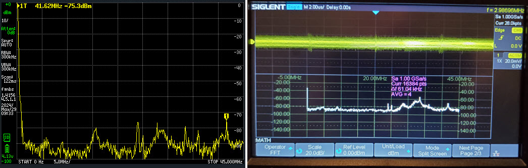
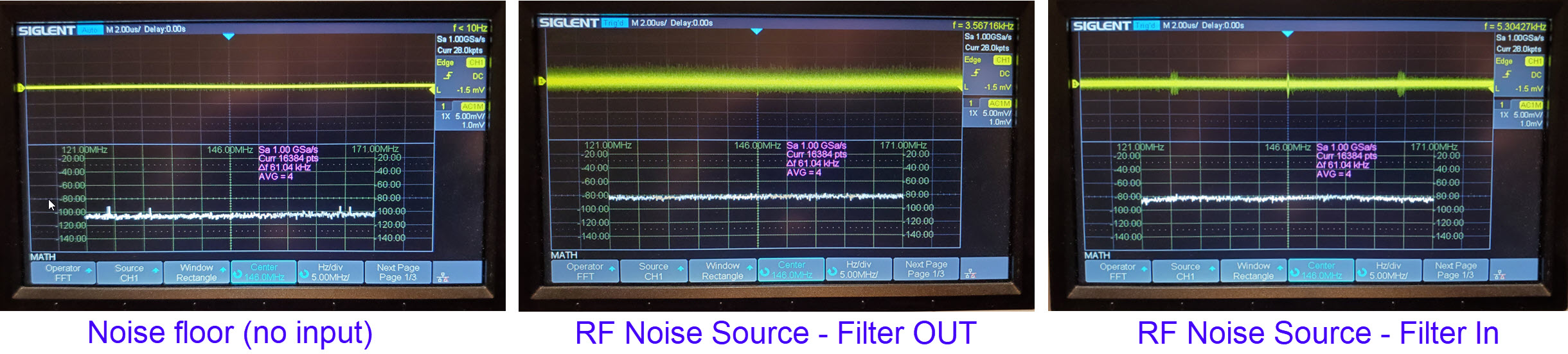
The first thing observed with this filter was a
noticeable increase in noise that appears in both oscilloscope and
tinySA measurements. The illustration above shows representative
tinySA and oscilloscope screens with the filter attached but no
stimulus. It can be guessed that the mess of wires and components on
the Mighty Mite
board were acting as an antenna.
The effect of inserting this particular low pass
filter in the signal path is clear at a glance. Both the tinySA Ultra
and oscilloscope displays show that power is preserved at the
fundamental frequency (essentially unchanged from its measurement with
no filter),
while all the observed harmonics are significantly suppressed. There is
no need to examine the numbers, but deltas range from approximately -50
to -60 dBc, thus confirming the conclusion of casual inspection. It was
reassuring finally to obtain one clearcut result from these somewhat tedious filter
measurements.
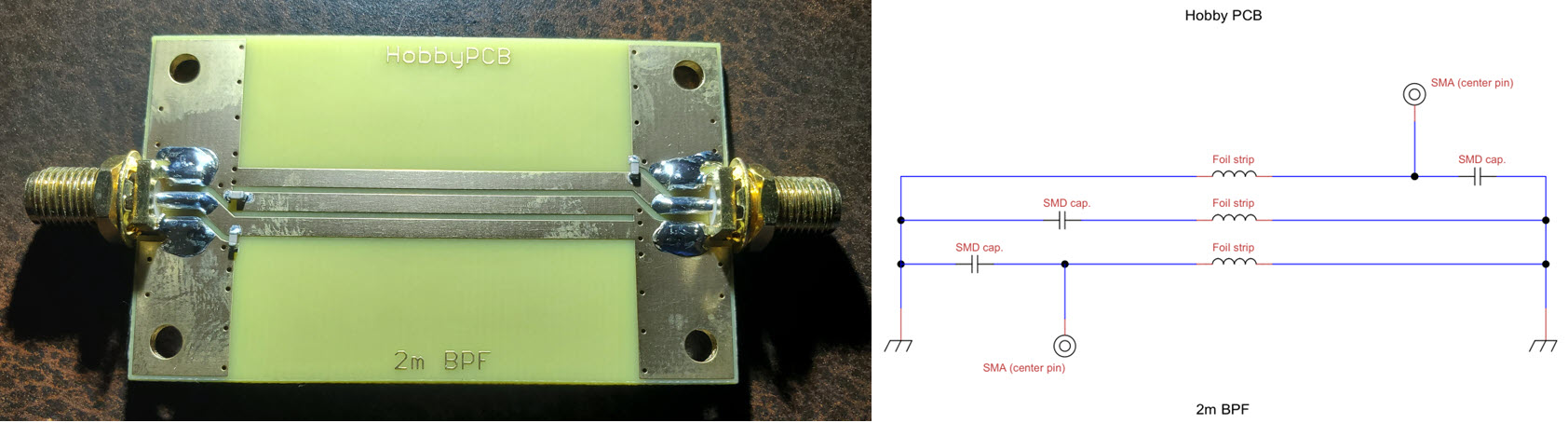
 Exercise 7: This exercise explored parameters of a
store-bought 144 MHz band pass filter, this one. The circuit diagram reproduced above is
unofficial
and may be inaccurate. It is my attempt to trace the circuit shown in
the photo.5 Based on the length and width of the foil
tracks, as measured with a millimeter rule, an on-line calculator yields the value 32 nH for each
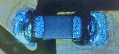
of the inductors. Components labeled ‘SMD cap.’ on the diagram were not
marked, and could not be measured in the circuit—See enlarged view at
right. (I was not
inclined to desolder them for measurement.)
Exercise 7: This exercise explored parameters of a
store-bought 144 MHz band pass filter, this one. The circuit diagram reproduced above is
unofficial
and may be inaccurate. It is my attempt to trace the circuit shown in
the photo.5 Based on the length and width of the foil
tracks, as measured with a millimeter rule, an on-line calculator yields the value 32 nH for each
of the inductors. Components labeled ‘SMD cap.’ on the diagram were not
marked, and could not be measured in the circuit—See enlarged view at
right. (I was not
inclined to desolder them for measurement.)
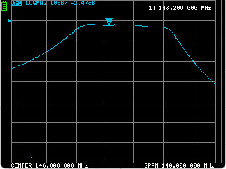
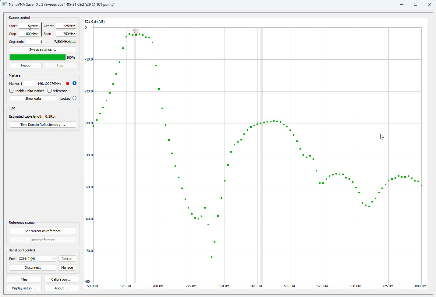
I first examined this filter using the NanoVNA and
subsequently tried a few things with a broad-spectrum RF noise source
and tinySA Ultra. For the NanoVNA observations, the filter was
connected between S11 and S21. Various frequency ranges were tried.
Testing a narrow frequency span resulted in a nearly flat line. I
wanted to see a bump, but this particular filter has a broad pass band.
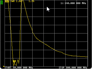
The screenshot (left) reflects one of many frequency
ranges tested. The display does not include labels for the vertical
scale. However, the NanoVNASaver computer application does indicate
ordinate values. Several measurements were made using the computer
application
as well. Those graphs will be omitted from this summary, partly
in the interest of space, but also because none of them resembled the
specification graphs on the HobbyPCB web page. Those graphs reflected an enormous frequency range (50 to 900
MHz)—I should have noticed!
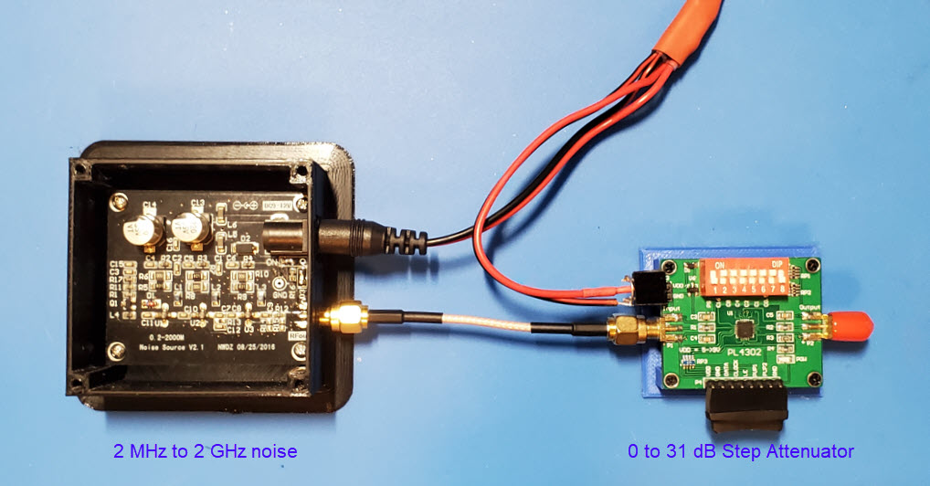
The stimulus configuration illustrated above
consists of a
broad-spectrum RF noise source, 2 MHz to 2 GHz, followed by a step
attenuator. In the photo the attenuator’s DIP switches are set to -31
dB. However, attenuation was subsequently changed to
-16 dB for this exercise, producing between -70 dBm and -60 dBm of
noise power. The attenuator’s output (rightmost SMA connector with red
cover) was connected to the 144 MHz bandpass filter using a double male
SMA adapter. In turn the filter’s output was connected to the tinySA
Ultra’s RF
↔ jack using another short RG-316 jumper. For background levels, the
filter was omitted and the step attenuator was connected directly to the
spectrum analyzer.
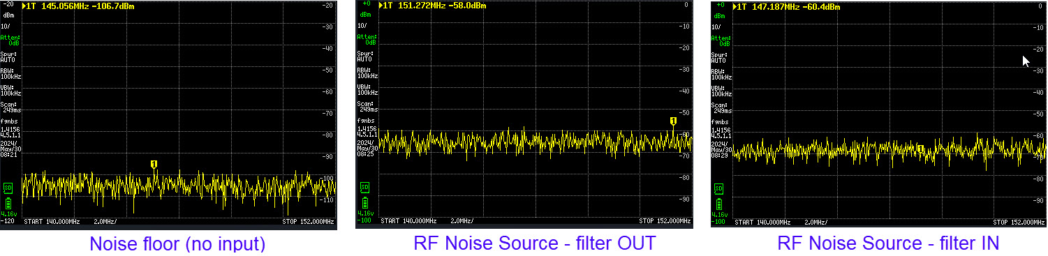
With no input at all (tinySA input not connected)
the noise floor was between -100 dBm and -110 dBm. Not surprisingly,
given the NanoVNA measurements and the published filter specification,
the noise remained flat across the tested frequency span with the band
pass filter in the chain. The level is slightly diminished with the
filter in, a few dB below the middle graph’s measurement. Not much can
be said about these noise measurements. Likely, the observed frequency
span is
too narrow. However, the original idea of these exercises was to
compare TinySA measurements with an oscilloscope’s math mode, so why
not!
Interestingly, absolute power levels are in
agreement between the oscilloscope and TinySA Ultra in this frequency
range. The oscilloscope’s vertical scale is more compressed than
tinySA’s. However, power is approximately the same, within display
resolution. The oscilloscope’s frequency span (50
MHz) is larger than in the tinySA screenshots.
A great many more observations were made than
were
recorded in screenshots or photos, and unfortunately direct comparisons
are not possible for each test condition. Before starting this exercise
I had expected to see a hole or a bump in the noise due to the filter.
No such effects were observed in any of the tests conducted, but stay
tuned!
Exercise 8: This exercise may be considered a ‘last gasp’
144 MHz filter study, having no relevance to the oscilloscope FFT
question. After reexamining the band pass filter’s specification graphs,
with particular attention to the abscissas, I thought it should be
possible to reproduce a spectrum display having the same shape by
suitable scaling and signal averaging. That turned out to be the case.
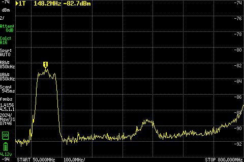
The TinySA Ultra screenshot above reflects a running
average of 16 sweeps through the 144 MHz filter. The RF noise source
was the same as in exercise 7, with the same attenuation settings, etc.
However the sweep spans 50 to 800 MHz and
the vertical (power) scale has been adjusted to 2 dBm/div with
auto-leveling. The larger of the two bumps is centered near the top of
the 2 meter ham band (marker 1). The smaller bump is around 3×
the pass band frequency.
Emboldened by success, if the preceding can be
regarded as such, I decided to have another go with the NanoVNA using
the same broad frequency range for the stimulus. The 144 MHz band pass
filter was connected between S11 and S21 as before.
OK the above graph is big! —Forget any concern for conserving space. As with the preceding
spectrum analyzer noise graph, the above reflects an average of 16
sweeps. In this case averaging makes no difference as the same points
are recorded on each sweep. I chose the ‘Gain’ format because the shape
was indistinguishable from the S21 log MAG plot. However, NanoVNASaver
plots both S11 and S21 log MAG graphs together and they overlap near
the interesting part. It was clearer to plot just S21 Gain. By the way,
the grey bands (vertical strips) in NanoVNASaver graphs represent ham
radio bands.
One of the NanoVNA screenshots resembled
the bottom product specification graph on the HobbyPCB page.
The part at marker 1 is
virtually identical in the comparison graph, while the right part of
the trace to 800 MHz was flat in the specification. However, I do not
know about
the measurement conditions or scale of the latter, which no doubt were
different. Throughout this exercise I have looked for similarities of
shape,
deliberately neglecting the meaning of measurements. In a sense the
objective was to prove that the 144 MHz band
pass filter was in fact a filter. The absence of a salient change
in noise power, as observed in the preceding exercise had led me to
wish for more demonstrable evidence. Similarities in form between the
graphs of this final exercise and the filter specifications would seem
to constitute persuasive evidence for
the supposition in question.
Endnotes
1. AKA math mode. FFT stands for Fast Fourier
Transform, a mathematical procedure for converting a time domain
function to
the frequency domain.
2. Power is RMS voltage squared divided by impedance.
63 mV P-P divided by 2*√2 = 22.27 mV RMS (or 0.02227 volts). 0.02227
volts squared divided by 50 ohms is .0000099225 watts (.0099225 mW).
[An easy-to-remember formula for RMS power in watts as a
function of peak to peak voltage is P = E2p-p
/ 8Z. The result is the same, of course, because (2√2)2 =
8.] Converting .0099225 mW to dBm,
10 times Log(.0099225) is -20.03, close enough. By
similar calculation, 200 mV corresponds to -10 dBm, and 20 mV to -30
dBm.
3. Oscilloscope: AC coupled, 50 ohms. FFT:
1 GSa/sec, 45 MHz swath of specturm, 214 bins. Display: 0
dBm reference, 20 dB per solid grid line, unless otherwise noted.
4. dBc stands for ‘decibels relative to carrier’.
5. The reverse side of the PCB (not pictured) has a foil covering to which the SMA jacks are soldered, making a common ground.
Project descriptions
on this page are intended for entertainment only.
The author makes no claim as to the accuracy or completeness of the
information presented. In no event will the author be liable for any
damages, lost effort, inability to carry out a similar project, or
to reproduce a claimed result, or anything else relating to a decision
to use the information on this page.