Billions
and Billions
Remembrance of
things past: Most people of my generation recall Carl Sagan’s
‘billions and billions’, pronounced with an
exaggerated hard ‘b’ sound, except that Carl Sagan didn’t actually
utter those words.1 The true source of this
memory was Johnny Carson spoofing Carl Sagan! Be that as it may, there
are billions of stars in our galaxy and billions of galaxies in the
universe, just as Carl Sagan said there are. Perhaps a lesser known
fact is that our amateur radio transmitters spew forth billions and
billions of photons per second. Indeed the word ‘billions’ is much too
small to express the numerosity of the energy packets that we routinely
cast into our world and beyond.
It is not necessary to have studied physics to know
that x-rays are more energetic than visible light—that’s why the dental
technician covers us with a heavy blanket before hastening from the
room to shoot the required annual image of our so-called ‘bite’.
Similarly we know that visible light is more energetic than microwaves,
which are more energetic than VHF/UHF, and so forth through high
frequencies, medium and long waves, all the way down to the Schumann
resonances.2 Come to think of it, a person
does not need to have studied physics in order to learn almost anything
about our universe nowadays. The answer can be found in Google 101 or
StartPage or DuckDuckGo or wherever you like.
Physics, or science in general, often deals with
numbers and I’ve learned over the years that many people are
uncomfortable with numbers. They are okay with reading the word
‘billion’ but the number 1,000,000,000 (which is the same thing) makes
them cringe. A sort of workaround for this problem is an extended set
of words for bigger and bigger quantities, trillion, quadrillion,
quintillion, and so forth. The same works in the other direction,
micro, nano, pico, femto, etc.3 But there
comes a point where you need numbers, as the words become awkward, like
working with Roman numerals—I’m writing this paragraph in MMXXIII.
Maybe the solution is to promise something. “If you
can tolerate a few numbers, I will tell you how many photons a 100 Watt
transmitter shoots forth per second at 7.150 MHz.” But wait, there is
no
need to suffer. With the admittedly unrealistic assumption
that the entire 100 Watts power is effectively radiated at the
specified frequency, I will state the answer to an absurd degree of
precision. It is
twenty-one octillion, one hundred seven septillion, five hundred
fifty-four sextillion, nine hundred sixty quintillion, thirty
quadrillion, ninety-five trillion, six hundred ninety billion, more or
less. How satisfying was that? —Not very!
Biting the numbers
bullet: We are ham radio operators, after all. We must deal with
some numbers, like how long to
cut the dipole wires, or how much reflected power our transmitter is
able to tolerate—oops! We must also have
passed a license exam, though that may have been in the distant past,
and it’s possible we could have forgotten some of those answers. Well,
surely we have not forgotten such fundamentals as the fact that
wavelength is inversely proportional to frequency. Though it may seem
less intuitive, it is just as simple to work out the immense number of
photons per second at 7.150 MHz, as it is to convert
frequency to wavelength, or vice versa. Instead of the speed of light,
a different constant of nature enters the picture. This one describes
how the energy of a photon varies with its frequency.
Planck’s constant is an exceedingly small
number. In ordinary decimal notation it is
0.000000000000000000000000000000000662607015 Joule-seconds. Scientists
and engineers use a more compact notation, 6.626 × 10⁻³⁴
J-s, but never mind that just yet.
The
energy of a photon is Planck’s
constant multiplied by its frequency in Hertz. You can see where
multiplying this miniscule number by a few billion isn’t
going to tip the scale very far! Now, one last piece of arithmetic
lore...
Dividing by a small number makes a large number. For example, dividing
by one-half is the same as multiplying by two. Dividing by one-tenth is
the same as multiplying by 10, and so forth. More to the point,
dividing power in Watts by the energy of a photon (at a given
frequency) gives the number of photons per second being generated. With
this one additional fact you can check my arithmetic on the 7.150 MHz
problem. —I have been known to be wrong.
Penetrating the mist:
It is one thing to calculate how many photons are generated, but how
many of them are getting through to Timbuctoo?—either
the
one in Mali, or the one in California. Stay tuned.
* * *
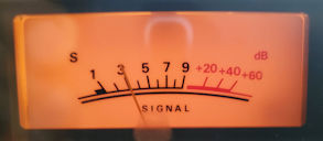 When the operator says you are 5-9 in Timbuctoo, it is best not to take
the report too literally. Surely every station cannot be 5-9 in
Timbuctoo! Alas, politeness has overtaken accuracy in the signal
reports business. Your true signal is more likely to be the one
illustrated pictorially on the left. For the sake of this exercise,
let’s assume that the transmitted signal is received as S3 in
Timbuctoo, and that the S-meter has been calibrated. The latter would
rarely be a safe assumption, but we have to start somewhere. According
to hamwaves.com,
a reading of S3 equates to -109 dBm at 50 ohms,
provided
that the S-meter is ‘well-designed’ and has been
calibrated for the high frequencies.4 But,
what does that mean?
When the operator says you are 5-9 in Timbuctoo, it is best not to take
the report too literally. Surely every station cannot be 5-9 in
Timbuctoo! Alas, politeness has overtaken accuracy in the signal
reports business. Your true signal is more likely to be the one
illustrated pictorially on the left. For the sake of this exercise,
let’s assume that the transmitted signal is received as S3 in
Timbuctoo, and that the S-meter has been calibrated. The latter would
rarely be a safe assumption, but we have to start somewhere. According
to hamwaves.com,
a reading of S3 equates to -109 dBm at 50 ohms,
provided
that the S-meter is ‘well-designed’ and has been
calibrated for the high frequencies.4 But,
what does that mean?
dBm to Watts:
First, observe that the letter ‘m’ in dBm stands for ‘milliwatt’.
That’s easy enough. However, at this point it becomes necessary to
introduce a swear word. If you already hang out with swear words, then
this one is not particularly fearsome. It is the word ‘logarithm’. More
precisely it is the common logarithm, where ‘common’ refers to base-10,
the number base that is commonly
used for counting things. The symbol dB (decibels) is nothing more than
ten times the base-10 logarithm of a number. One of the shortcuts we
learn in ham radio is that a 3dB power gain corresponds to doubling the
power. Doubling, of course, is the same as multiplying by 2, and the
base-10 logarithm of 2 is approximately 0.3, which multiplied by 10
makes 3 dB.
Before losing track let’s return to the S-meter
reading. Our signal was S3, or -109 dBm in Timbuctoo. Although these
intermediate steps are probably explanation overkill, to be clear, -109
dB means
that the logarithm of the power ratio is -10.9 (divide dB by 10). To
work backwards from dBm to power, multiply 1 milliwatt (.001 Watts) by
10-10.9. As may be expected, the result is a very
small quantity. Expressed to an absurd number of
decimal places the value works out to be
.0000000000000125892541179416721... Watts. Believe it or not, there is
a prefix for this miniscule amount of power. Rounded to 3 places, it is
12.6 femtowatts.
The number of photons per second impinging upon the
receiver is this small number divided by the previously computed energy
of a photon at 7.15 MHz (Planck's constant multiplied by 7,150,000 Hz).
Drum roll... The number is 2,657,283,732,002 (more or less). In words,
it is two trillion, six hundred fifty-seven billion, two hundred
eighty-three million, seven hundred thirty-two thousand and two photons
per second. In contrast to the enormous number that was computed for
the transmit power, this one is small enough to be dollars instead of
photons! As dollars it would be a small fraction of the US national
debt.5
Photons per unit
area per second: Counting energy packets that equate to an
S-meter reading was messy to say the least. However, to continue in the
spirit of glorifying big numbers, and expressing them to preposterous
precision, the exercise can be carried one step
further. The concept is called ‘photon flux’. Stay tuned.
* * *
Here comes another swear word, ‘isotropic’. It is
the ‘i’ in dBi, in case you happen to have seen that symbol. The term
‘isotropic’ means ‘same in every direction’. Ham radio antennas are not isotropic. On the other hand,
the gain of a directional antenna may be conveniently expressed in dBi
units, or decibels over isotropic. For example, the gain of a dipole
(in free space) is 2.15 dBi. The dipole itself often serves as a comparison
reference for expressing the gain of other antenna types. Decibels
(logarithms)
are additive, so if a Yagi antenna has 8 dB forward gain with respect
to a dipole, it would be the same to say its forward gain is
approximately 10
dBi. Bear in mind that real antennas are not ideal antennas. Real
antennas are affected by their height above ground, and countless other
installation-specific environmental factors.
The word isotropic
plays an important role in a concept called the ‘inverse square law’. I
don’t want to make more of this than is obvious. If a substance
emanates outwards from a point equally in all directions, then at any
given distance the substance will be dispersed evenly on the surface of
an imaginary sphere whose radius is said distance. In school
we either deduced or memorized (and then quickly forgot) the formula
for the surface area of a sphere 4πr2, where r stands for its radius. In the
inverse square law, the letter d
(distance) replaces r
(radius) in this expression.
Putting the inverse square law together with the count of photons at
the source leads to the concept of photon flux,
sometimes denoted by an uppercase Φ.
Flux is simply the number of photons per second per unit area at a given distance
from the source.
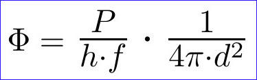 At this point it may be necessary to
apologize for sneaking in a potentially frightening formula. But
each of
the symbols in the formula stands for something that has been explained
already, P for power in
Watts, h for Planck’s
constant, f for frequency in
Hz, and d for distance in
whatever units you want. If distance is specified in meters, then area
will be meters squared, and so forth. As illustrated here, the photon
flux calculation assumes isotropy. For convenience the formula has been
split into sub-expressions to emphasize the radiative source (left) and
its inverse square diminution (right).6
At this point it may be necessary to
apologize for sneaking in a potentially frightening formula. But
each of
the symbols in the formula stands for something that has been explained
already, P for power in
Watts, h for Planck’s
constant, f for frequency in
Hz, and d for distance in
whatever units you want. If distance is specified in meters, then area
will be meters squared, and so forth. As illustrated here, the photon
flux calculation assumes isotropy. For convenience the formula has been
split into sub-expressions to emphasize the radiative source (left) and
its inverse square diminution (right).6
Effective area:
Ham radio transmit antennas are not isotropic. And receive antennas
don’t resemble a chunk from a spherical collecting surface. Moreover,
who’s going to climb an antenna tower with a tape measure in hand, and
what
would they
do with it if they did? As it happens, nobody has to climb the tower,
or measure antenna parts because, according to this page, “the effective
area of an antenna ... is the area of the idealized antenna that
absorbs as much net power from the incoming wave as the actual antenna
[does].” With a few lines of symbol manipulation that same page deduces
the effective area of a (Hertzian) dipole7
to be three times the wavelength squared divided by 8π.
In the spirit of fudging when expedient to do so, I will use this
expression to compute the area of the make-believe receive antenna in
Timbuctoo.
The frequency 7.150 MHz falls in the 40 meter ham radio
band. At this frequency the free-space
wavelength is closer to 41.9
meters, but no-matter. Let’s say λ ≈ 40 meters. That should be close
enough. Applying the effective area formula from the preceding
paragraph we get approximately 190 m² for the area of the receive
antenna. (Check me!) At this point it is time to let go the excessive
precision of photon counts. Dividing 2,657 billion by 190 meters
squared obtains a flux of approximately 14 billion photons per second
per meter squared at the receiving antenna. Hmm. Now I’m thinking of
even crazier calculations, like given the distance to Timbuctoo, how
would the antenna’s measured
gain compare to the isotropic flux calculation for the same distance.
Of course it would not be necessary to use photon flux in the
calculation, as the same comparison can be done with power in Watts.
Big numbers
on this page are just for fun.
 Wrap up and wind
down:
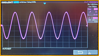
Waves are everywhere, especially in ham radio,
long waves, medium waves, shortwaves, waves of voltage and current on
the transmission line and antenna, electric and magnetic components of
the RF wave, in-phase and quadrature to the SDR, and so on.
Wrap up and wind
down:
Waves are everywhere, especially in ham radio,
long waves, medium waves, shortwaves, waves of voltage and current on
the transmission line and antenna, electric and magnetic components of
the RF wave, in-phase and quadrature to the SDR, and so on.
Waves correspond to the natural way of thinking
about radio, as we know it. They form a conceptualization that works,
and has passed the test of time. Nevertheless it is fun to contemplate
the magic of radio in a different way, to visualize billions and
billions of infinitesimal beadies shooting forth, bouncing and
penetrating and otherwise wending their way to remote and exotic places.
1. Chapter 1 in Sagan’s posthumous Billions & Billions... Sagan did intentionally
pronounce the word with a hard ‘b’ to emphasize that he was not saying
‘millions’.
2. https://en.wikipedia.org/wiki/Schumann_resonances
3. https://www.varsitytutors.com/hotmath/hotmath_help/topics/big-and-small-numbers
4. S-meter calibration differs for VHF/UHF. For
example, S9 at HF translates to -73 dBm at 50 ohms, while for VHF/UHF
it is -93 dBm.
5. 8.4% at the time of this writing (https://www.usdebtclock.org/).
6. In the flux formula, frequency is sometimes
expressed as the speed of light divided by wavelength (f = C/λ), which puts wavelength in
the numerator and the constant C in the denominator.
7. Directivity = 3/2.
Project descriptions on this page are intended for entertainment only.
The author makes no claim as to the accuracy or completeness of the
information presented. In no event will the author be liable for any
damages, lost effort, inability to carry out a similar project, or to
reproduce a claimed result, or anything else relating to a decision to
use the information on this page.